\(\renewcommand\AA{\unicode{x212B}}\)

Inelastic Data Manipulation¶

Overview ¶

The Inelastic Data Manipulation interface provides Processes for manipulating reduced data from, for example, Indirect Data Reduction and Direct Reduction routines or S(Q, w). The output data can then be used for analysis by processes in, for example, the Inelastic QENS Fitting and Inelastic Bayes Fitting interfaces.

../../_images/Data_Manipulation_interface.png

Action Buttons ¶

Settings: Opens the Settings GUI which allows you to customize the settings for the Inelastic interfaces.

?: Opens this help page.
Py: Exports a Python script which will replicate the processing done by the current tab.
Manage Directories: Opens the Manage Directories dialog allowing you to change your search directories and default save directory and enable/disable data archive search.

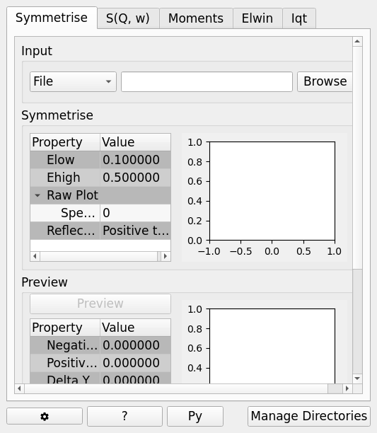
Symmetrise ¶

This tab allows you to take an asymmetric reduced file (_red.nxs) and symmetrise it about the Y axis.

The center of energy in the Y axis (E=0) is indicated by a solid red line. Two green vertical dashed lines can be moved to change the value of \(E_{low}\) and \(E_{high}\), which is the range of energies used to symmetrise the spectra. Additionally, two horizontal blue dotted lines can be moved to help in selecting a range that prevents rigged curves when the spectra is symmetrised.

The curve can be symmetrised using either side of the spectra by changing the Reflect Type property. This choice influences the direction onto which the spectra is symmetrised. Note that \(E_{low}\) represents the lowest value on the range, so when the spectra is on the positive side, \(E_{low}\) will be closer to the centre while in the negative side \(E_{low}\) will be farther from the centre. The following methods are available on the Reflect Type property:

Positive to Negative (default): the range of the positive values between \(E_{low}\) and \(E_{high}\) is reflected about the Y axis and replaces the corresponding values in the negative side of the spectra. The curve which ranges between \(\pm|E_{low}|\) is not modified.
Negative to Positive: the range of the negative values between \(-E_{low}\) and \(-E_{high}\) is reflected about the Y axis and replaces the corresponding values in the positive side of the spectra. The curve which ranges between \(\pm|E_{high}|\) is not modified.

../../_images/Data_Manipulation_tabSymmetrise_widget.png

Symmetrise Options ¶

Input: Allows you to select a reduced NeXus file (_red.nxs) or workspace (_red) as the input to the algorithm.
ELow & EHigh: Sets the energy range that is to be reflected about \(y=0\).
Reflect Type: Whether to do Positive to Negative or Negative to Positive reflection.
Spectrum No: Changes the spectrum shown in the preview plots.
XRange: Changes the range of the preview plot, this can be useful for inspecting the curve before running the algorithm.
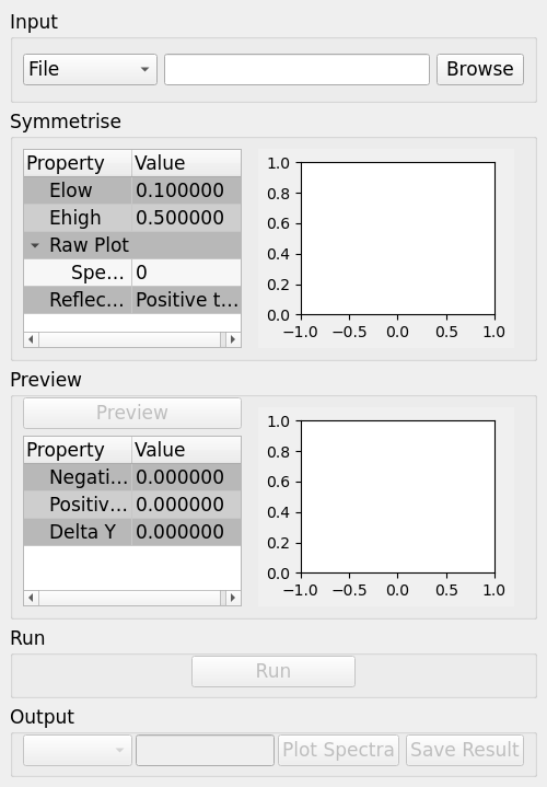
Preview: This button will update the preview plot and parameters under the Preview section.
Run: Runs the processing configured on the current tab.
Plot Spectra: If enabled, it will plot the selected workspace indices in the selected output workspace.
Save Result: If enabled the result will be saved as a NeXus file in the default save directory.

Preview ¶

The preview section shows what a given spectra in the input will look like after it has been symmetrised and gives an idea of how well the value of \(E_{low}\) fits the curve on both sides of the peak.

Negative Y: The value of \(y\) at \(x=-|E_{low}|\) on Positive to Negative or at \(x=-|E_{high}|\) on Negative to Positive.
Positive Y: The value of \(y\) at \(x=|E_{low}|\) on Positive to Negative or at \(x=|E_{high}|\) on Negative to Positive.
Delta Y: The difference between Negative and Positive Y. Typically this should be as close to zero as possible.

Symmetrise Example Workflow ¶

The Symmetrise tab operates on _red files. The file used in this workflow can be produced using the 26176 run number on the ISIS Energy Transfer tab. The instrument used to produce this file is IRIS, the analyser is graphite and the reflection is 002. See the ISIS Energy Transfer Example Workflow.

In the Input box, load the file named iris26176_graphite002_red. This will automatically plot the data on the first mini-plot.
Move the green slider located at x = 0.5 to be at x = 0.4.
Click Preview. This will update the Preview properties and the neighbouring mini-plot.
Click Run and wait for the interface to finish processing. This will run the Symmetrise algorithm. The output workspace is called iris26176_graphite002_sym_pn_red.
Click Plot Spectra to produce a spectra plot of the output workspace. Other indices can be plotted by entering indices in the box next to the Plot Spectra button. For example, entering indices 0-2,4,6-7 will plot the spectra with workspace indices 0, 1, 2, 4, 6 and 7.

Go to the S(Q, w) Example Workflow.

S(Q, w)¶

Provides an interface for running the SofQW algorithm SofQWNormalisedPolygon.

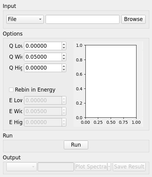
../../_images/Data_Manipulation_tabSQw_widget.png

S(Q, w) Options ¶

Input: Allows you to select a reduced NeXus file (_red.nxs) or workspace (_red) as the input to the algorithm. An automatic contour plot of _rqw will be plotted in the preview plot once a file has finished loading.
Q Low, Q Width & Q High: Q binning parameters that are passed to the SofQW3 algorithm. The low and high values can be determined using the neighbouring contour plot. The default values given show the Q range where there is data in the reduced workspace and these values cannot be changed.
Rebin in Energy: If enabled the data will first be rebinned in energy before being passed to the SofQW algorithm.
E Low, E Width & E High: The energy rebinning parameters. The low and high values can be determined using the neighbouring contour plot.
Run: Runs the processing configured on the current tab.
Plot Spectra: If enabled, it will plot the selected workspace indices in the selected output workspace.
Open Slice Viewer: If enabled, it will open the slice viewer for the selected output workspace.
Save Result: If enabled the result will be saved as a NeXus file in the default save directory.

S(Q, w) Example Workflow ¶

The S(Q, w) tab operates on _red files. The file used in this workflow can be produced using the 26176 run number on the ISIS Energy Transfer tab. The instrument used to produce this file is IRIS, the analyser is graphite and the reflection is 002. See the ISIS Energy Transfer Example Workflow.

In the Input box, load the file named iris26176_graphite002_red. This will automatically plot the data as a contour plot within the interface.
Set the Q Low, Q Width and Q High to be 0.5, 0.05 and 1.8. These values are read from the contour plot.
Tick Rebin in Energy.
Set the E Low, E Width and E High to be -0.5, 0.005 and 0.5. Again, these values should be read from the contour plot.
Click Run and wait for the interface to finish processing. This will perform an energy rebin before performing the SofQW algorithm. The output workspace ends with suffix _sqw and is called iris26176_graphite002_sqw.
Enter a list of workspace indices in the output options (e.g. 0-2,4,6-7) and then click Plot Spectra to plot spectra from the output workspace.

Click the down arrow on the Plot Spectra button, and select Open Slice Viewer. This will open a slice viewer window for the output workspace.
Choose a default save directory and then click Save Result to save the output workspace. The _sqw file is used in the Moments Example Workflow.

Moments ¶

This interface uses the SofQWMoments algorithm to calculate the \(n^{th}\) moment of an \(S(Q, \omega)\) workspace created by the SofQW tab.

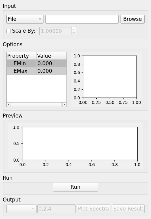
Moments Options ¶

Input: Allows you to select an \(S(Q, \omega)\) file (_sqw.nxs) or workspace (_sqw) as the input to the algorithm.
Scale By: Used to set an optional scale factor by which to scale the output of the algorithm.
EMin & EMax: Used to set the energy range of the sample that the algorithm will use for processing.
Run: Runs the processing configured on the current tab.
Plot Spectra: If enabled, it will plot the selected workspace indices in the selected output workspace.
Save Result: If enabled the result will be saved as a NeXus file in the default save directory.

Moments Example Workflow ¶

The Moments tab operates on _sqw files. The file used in this workflow is produced during the S(Q, w) Example Workflow.

In the Input box, load the file named irs26176_graphite002_sqw. This will automatically plot the data in the first mini-plot.
Drag the blue sliders on the mini-plot so they are x=-0.4 and x=0.4.
Click Run and wait for the interface to finish processing. This will run the SofQWMoments algorithm. The output workspace ends with suffix _moments and is called iris26176_graphite002_moments.

Elwin ¶

Provides an interface for the ElasticWindow algorithm, with the option of selecting the range to integrate over as well as the background range. An on-screen plot is also provided.

For workspaces that have a sample log, or have a sample log file available in the Mantid data search paths that contains the sample environment information the ELF workspace can also be normalised to the lowest temperature run in the range of input files.

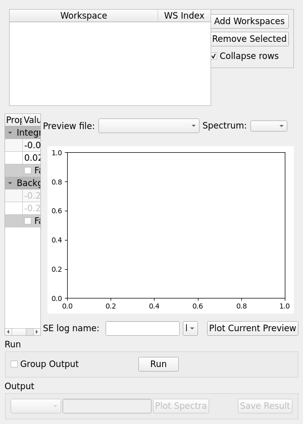
../../_images/Data_Manipulation_tabElwin_widget.png

Elwin Options ¶

File or Workspace: Choose to load data from a file or a workspace by using this dropdown menu. See image below for demonstration of how to load files using either option.

Input File: Specify a range of input files that are either reduced (_red.nxs) or \(S(Q, \omega)\).
Group Input: The ElasticWindowMultiple algorithm is performed on the input files and returns a group workspace as the output. This option, if unchecked, will ungroup these output workspaces.
Load History: If unchecked the input workspace will be loaded without it’s history.
Integration Range: The energy range over which to integrate the values.
Background Subtraction: If checked a background will be calculated and subtracted from the raw data.
Background Range: The energy range over which a background is calculated which is subtracted from the raw data.
Normalise to Lowest Temp: If checked the raw files will be normalised to the run with the lowest temperature, to do this there must be a valid sample environment entry in the sample logs for each of the input files.
SE log name: The name of the sample environment log entry in the input files sample logs (defaults to ‘sample’).
SE log value: The value to be taken from the “SE log name” data series (defaults to the specified value in the instrument parameters file, and in the absence of such specification, defaults to “last value”)
Preview File: The workspace currently active in the preview plot.
Spectrum: Changes the spectrum displayed in the preview plot.
Plot Current Preview: Plots the currently selected preview plot in a separate external window
Run: Runs the processing configured on the current tab.
Plot Spectra: If enabled, it will plot the selected workspace indices in the selected output workspace.
Save Result: Saves the result in the default save directory.

Elwin Example Workflow ¶

The Elwin tab operates on _red and _sqw files. The files used in this workflow can be produced using the run numbers 104371-104375 on the Indirect Data Reduction interface in the ISIS Energy Transfer tab. The instrument used to produce these files is OSIRIS, the analyser is graphite and the reflection is 002.

Untick the Load History checkbox next to the file selector if you want to load your data without history.
Click Browse and select the files osiris104371_graphite002_red, osiris104372_graphite002_red, osiris104373_graphite002_red, osiris104374_graphite002_red and osiris104375_graphite002_red. Load these files and they will be plotted in the mini-plot automatically.
The workspace and spectrum displayed in the mini-plot can be changed using the combobox and spinbox seen directly above the mini-plot.
You may opt to change the x range of the mini-plot by changing the Integration Range, or by sliding the blue lines seen on the mini-plot using the cursor. For the purpose of this demonstration, use the default x range.
Tick Normalise to Lowest Temp. This option will produce an extra workspace with end suffix _elt. However, for this to work the input workspaces must have a temperature. See the description above for more information.
Click Plot Current Preview if you want a larger plot of the mini-plot.
Click Run and wait for the interface to finish processing. This should generate four workspaces ending in _eq, _eq2, _elf and _elt.
In the Output section, select the workspace ending with _eq and then choose some workspace indices (e.g. 0-2,4). Click Plot Spectra to plot the spectrum from the selected workspace.
Choose a default save directory and then click Save Result to save the output workspaces. The workspace ending in _eq will be used in the MSD Fit Example Workflow.

I(Q, t)¶

Given sample and resolution inputs, carries out a fit as per the theory detailed in the TransformToIqt algorithm.

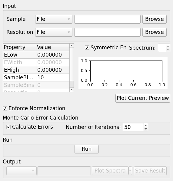
../../_images/Data_Manipulation_tabIqt_widget.png

I(Q, t) Options ¶

Sample: Either a reduced file (_red.nxs) or workspace (_red) or an \(S(Q, \omega)\) file (_sqw.nxs) or workspace (_sqw).
Resolution: Either a resolution file (_res.nxs) or workspace (_res) or an \(S(Q, \omega)\) file (_sqw.nxs) or workspace (_sqw).
ELow, EHigh: The rebinning range.
Enforce Normalization: The LHSWorkspace from the output from ExtractFFTSpectrum v1 is used in both branches to perform the final workspace division and the two intermediate workspace divisions are skipped by unchecking this option.
SampleBinning: The number of neighbouring bins are summed.
Symmetric Energy Range: Untick to allow an asymmetric energy range.
Spectrum: Changes the spectrum displayed in the preview plot.
Plot Current Preview: Plots the currently selected preview plot in a separate external window
Calculate Errors: The calculation of errors using a Monte Carlo implementation can be skipped by unchecking this option.
Number Of Iterations: The number of iterations to perform in the Monte Carlo routine for error calculation in I(Q,t).
Run: Runs the processing configured on the current tab.
Plot Spectra: If enabled, it will plot the selected workspace indices in the selected output workspace.
Plot Tiled: Generates a tiled plot containing the selected workspace indices. This option is accessed via the down arrow on the Plot Spectra button.
Save Result: Saves the result workspace in the default save directory.

I(Q, t) Example Workflow ¶

The I(Q, t) tab allows _red and _sqw for it’s sample file, and allows _red, _sqw and _res for the resolution file. The sample file used in this workflow can be produced using the run number 26176 on the Indirect Data Reduction interface in the ISIS Energy Transfer tab. The resolution file is created in the ISIS Calibration tab using the run number 26173. The instrument used to produce these files is IRIS, the analyser is graphite and the reflection is 002.

Click Browse for the sample and select the file iris26176_graphite002_red. Then click Browse for the resolution and select the file iris26173_graphite002_res.
Change the SampleBinning variable to be 5. Changing this will calculate values for the EWidth, SampleBins and ResolutionBins variables automatically by using the TransformToIqt algorithm where the BinReductionFactor is given by the SampleBinning value. The SampleBinning value must be low enough for the ResolutionBins to be at least 5. A description of this option can be found in the A note on Binning section.
Untick Calculate Errors if you do not want to calculate the errors for the output workspace which ends with the suffix _iqt.
Click Run and wait for the interface to finish processing. This should generate a workspace ending with a suffix _iqt.
In the Output section, select some workspace indices (e.g.0-2,4,6) for a tiled plot and then click the down arrow on the Plot Spectra button before clicking Plot Tiled.
Choose a default save directory and then click Save Result to save the _iqt workspace. This workspace will be used in the I(Q, t) Fit Example Workflow.

A note on Binning ¶

The bin width is determined from the energy range and the sample binning factor. The number of bins is automatically calculated based on the SampleBinning specified. The width is determined from the width of the range divided by the number of bins.

The following binning parameters cannot be modified by the user and are instead automatically calculated through the TransformToIqt algorithm once a valid resolution file has been loaded. The calculated binning parameters are displayed alongside the binning options:

EWidth: The calculated bin width.
SampleBins: The number of bins in the sample after rebinning.
ResolutionBins: The number of bins in the resolution after rebinning. Typically this should be at least 5 and a warning will be shown if it is less.

Categories: Interfaces | Inelastic